Machine learning

Video diffusion: learning to generate motion

A practical introduction to video diffusion, with equations, original diagrams, and a small experiment in learning to see motion.

September 24, 20265 min readLabbook

Table of contents6 sections

Imagine filming a blue ball rolling across a desk. A convincing generated clip must do more than draw a beautiful ball: its color should persist, its shadow should follow it, and its position should change in a plausible way. These requirements make video a useful test of what a generative model has learned about a scene.

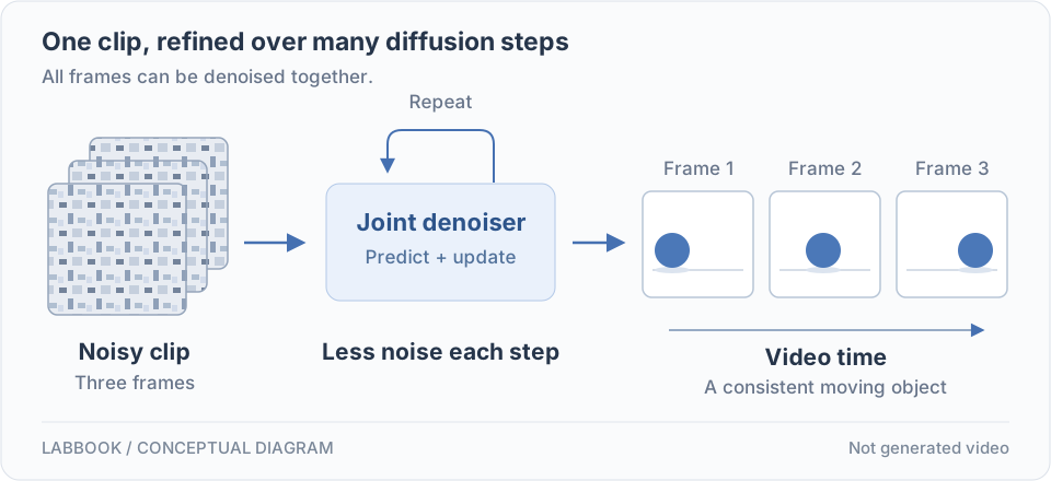
This note builds a working picture of video diffusion through five questions: what gets corrupted, how frames communicate, where the model spends computation, how sampling proceeds, and what counts as a successful result. The diagrams are conceptual sketches, not outputs from a trained model.

1. Start with a noisy clip

Let $x_0$ denote a clean clip with $F$ frames. The diffusion index $t$ describes a noise level; it is separate from the frame index. A familiar Gaussian corruption rule is

$$x_t = \sqrt{\bar\alpha_t}\,x_0 + \sqrt{1-\bar\alpha_t}\,\epsilon,
\qquad \epsilon\sim\mathcal N(0,I).$$

Here $\bar\alpha_t=\prod_{s=1}^{t}(1-\beta_s)$ , and the schedule $\beta_s$ controls noise accumulation. During training, the clean example supplies a known noise target. One common objective, shown with conditioning information $c$ , is

$$\mathcal L(\theta)=\mathbb E_{x_0,t,\epsilon,c}
\left[\left\|\epsilon-\epsilon_\theta(x_t,t,c)\right\|_2^2\right].$$

The network learns to predict the corruption at many noise levels. Generation then starts from noise and repeatedly applies a sampler using those predictions. This is the noise-prediction formulation associated with DDPM, extended here to a conditional clip tensor.

A noisy three-frame clip passes through repeated joint denoising steps to become a sequence showing a ball moving right. — Figure 1. Diffusion steps refine the whole clip. Moving from frame 1 to frame 3 is a different axis from moving from noise to a clean sample.

2. Give frames a shared context

Sampling each frame independently leaves their relationship unspecified. A model needs a route for information to travel across the clip. In Video Diffusion Models, Ho and colleagues interleave spatial and temporal attention in a video U-Net.

Spatial attention connects locations within one frame. Temporal attention connects frame positions along the time axis, treating spatial positions as separate groups. Alternating the two lets information move through both dimensions without constructing one enormous attention matrix over every location in every frame. This is one architectural choice, rather than a requirement of diffusion itself.

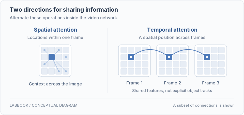
Two diagrams contrast attention among patches inside one frame with attention between the same spatial position in three frames. — Figure 2. A schematic of factorized attention. The temporal connections show feature communication, not an explicit trajectory tracker.

For the rolling ball, this distinction matters. A temporal block does not automatically know which pixel belongs to the ball after it moves. Spatial processing and learned features must help make that correspondence useful. Treat attention as a mechanism for sharing evidence, not a guarantee that identity or physical behavior will remain correct.

3. Decide where computation happens

A clip multiplies the amount of visual data a model must process. Latent Diffusion Models offer an important image-generation idea: learn a compressed representation with an autoencoder, perform diffusion there, and decode the result afterward. The representation reduces the spatial workload, while its reconstruction quality limits which details can survive.

For a video system, that suggests a useful diagnostic: inspect the representation before blaming the generator. If encoding and decoding a real clip already damage a small moving object, denoising cannot be expected to recover all of that information reliably. This is an experimental deduction from the bottleneck, not a claim that every video model uses the same encoder.

Another way to divide the workload is a cascade. Imagen Video combines a base video model with spatial and temporal super-resolution models. The base establishes a coarse clip; later stages increase resolution or frame rate. Latent representations and cascades answer different design questions, so they should not be treated as interchangeable labels.

4. Choose the sampling path deliberately

The denoiser and the sampler have different jobs. The network predicts a quantity at a noise level. The sampler uses it to choose the next state. DDIM shows how alternative sampling trajectories can use the same training objective and trade sampling effort against quality.

For the notation above, a predicted clean sample is

$$\hat x_0 = \frac{x_t-\sqrt{1-\bar\alpha_t}\,
\epsilon_\theta(x_t,t,c)}{\sqrt{\bar\alpha_t}}.$$

This estimate is an ingredient of an update, not a complete sampler. The following sketch keeps that boundary explicit:

clip = gaussian_noise(clip_shape, seed)
conditioning = encode_prompt(prompt)

for current, following in schedule_pairs:
    prediction = denoiser(clip, current, conditioning)
    clip = sampler.step(prediction, current, following, clip)

video = decode_if_latent(clip)

The schedule, prediction parameterization, and sampler must agree. A text prompt supplies conditioning; it does not specify a unique motion path. For an experiment, keep the prompt and initial seed fixed while changing the number of sampling steps. Then compare several seeds before drawing conclusions: a single attractive clip can hide substantial variation in behavior. This controlled comparison is a proposed workflow, rather than a benchmark result.

5. Watch the failures, then design an experiment

For the desk example, write down observable checks before generating anything. Does the ball keep its shape? Does the shadow move consistently? Does it travel in the requested direction? Does the background remain stable? Separating these questions makes an unsuccessful clip more informative than a single judgment of “looks wrong.”

Fréchet Video Distance was introduced to assess generated video distributions using video features, with evidence of correlation with human judgments. It provides a useful aggregate view, but an aggregate comparison does not tell you whether a particular ball passed behind the correct object. Pair distribution-level evaluation with task-specific inspection.

A small study could compare three conditions: a stationary ball, a rolling ball, and a ball temporarily hidden behind a box. Keep the camera description constant. Save the prompt, seed, model version, resolution, frame rate, sampler, and runtime alongside each result. Inspect ordinary playback first, then pause at the moment of occlusion.

The interesting outcome is not necessarily the prettiest clip. If identity changes only after occlusion, that points to a different weakness than flicker throughout the background. Record the failure and the next experiment together. Over time, the notebook becomes a collection of testable observations about motion, representation, and control.

References

Ho, Jain, and Abbeel. Denoising Diffusion Probabilistic Models, 2020.
Ho et al. Video Diffusion Models, 2022.
Rombach et al. High-Resolution Image Synthesis with Latent Diffusion Models, 2022.
Song, Meng, and Ermon. Denoising Diffusion Implicit Models, 2021.
Ho et al. Imagen Video: High Definition Video Generation with Diffusion Models, 2022.
Unterthiner et al. Towards Accurate Generative Models of Video: A New Metric & Challenges, 2018.

An original Labbook sample with custom illustrations. Reading-layout inspiration: Lilian Weng's technical essays.